LLMs today are quite large and the size of these LLMs both in terms of memory and computation is only increasing. At the same time, demand for running the LLMs on small devices is equally increasing. If you wish to run a modern-day LLM on a laptop or a mobile phone or even a web browser, then you need to quantize the LLM — be it pre-trained or fine-tuned.

This coding tutorial is a walkthrough of two simple quantization methods that are building blocks to advanced methods like GPTQ. If you are someone who wishes to dip your hands into simple concepts before moving on to advanced concepts, please stay tuned.

Note: An understanding of quantization types and floating point representations from my previous article available here is needed for this hands-on tutorial.

LLM Model

Though there are a variety of models to choose from these days, I found that the latest gemma-2b model was large for this demonstration and proved challenging to run on a colab notebook (without sophisticated quantization frameworks). As we are implementing naive quantization methods, let's step back and choose a much smaller model. I have gone for flan-t5-small model.

Related Resources

• Code: The code for this notebook can be found here
• Visual explanation. If you are like me and would prefer a visual explanation, please check it out:

Absolute Max Quantization

In absolute max quantization, we compute the maximum of the absolute values of all elements in the input and normalize the input with it, followed by scaling up and rounding to the nearest whole number as indicated below.

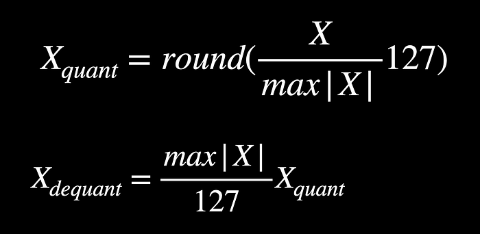
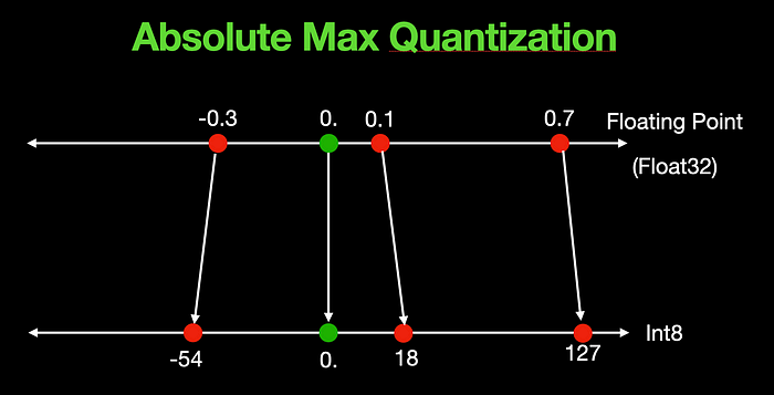
Above is a quantization example for an input of [-0.3, 0., 0.1, 0.7]. Zero at the input always maps to zero at the output irrespective of the input values.

Implementation

The above idea can be implemented by 4 lines of code as below.

def absmax_quantize(ip):
# Calculate scale
scale = 127 / torch.max(torch.abs(ip))
# Quantize
ip_quant = (scale * ip).round()
# Dequantize
ip_dequant = ip_quant / scale
return ip_quant.to(torch.int8), ip_dequant

Zero Point Quantization

In the case of zero point quantization, the zero value for the quantized result is dynamic and computed based on the input vector or tensor. For the same example of [-0.3, 0., 0.1, 0.7], the zero point is skewed towards the left and takes a value of -52 as shown below.

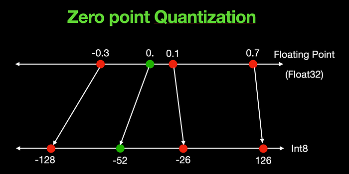
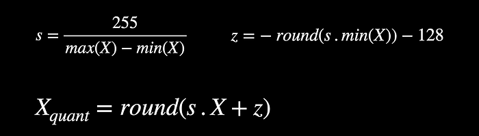
The above are the equations for zero point quantization which carries an additional z parameter for zero point calculation and hence the name.

Implementation

def zeropoint_quantize(ip):
# Calculate scale
ip_range = torch.max(ip) - torch.min(ip)
ip_range = 1 if ip_range == 0 else ip_range
scale = 255 / ip_range
# calculate zeropoint
zeropoint = (-scale * torch.min(ip) - 128).round()
# quantize by rounding
ip_quant = torch.clip((ip * scale + zeropoint).round(), -128, 127)
# dequantize
ip_dequant = (ip_quant - zeropoint) / scale
return ip_quant.to(torch.int8), ip_dequant

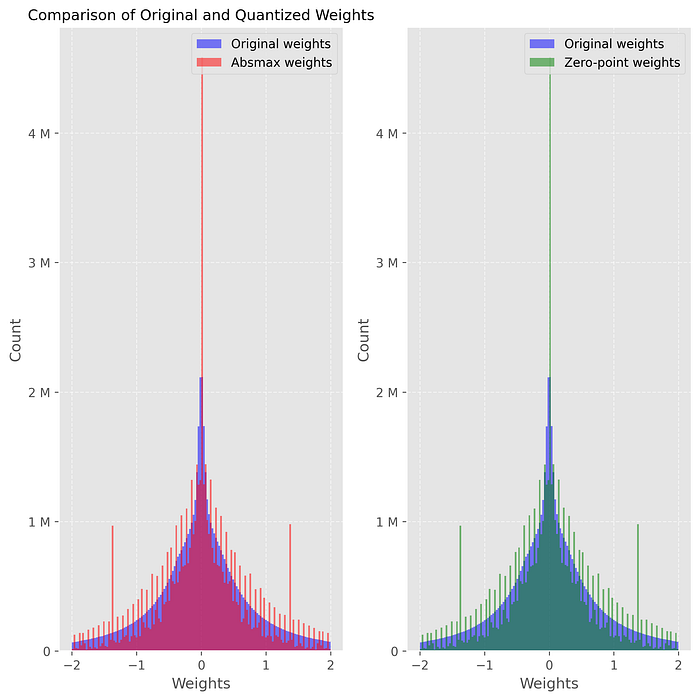
Comparison of Quantized weights

As we can see from below, after quantizing and dequantizing, the distribution of the weights is slightly different from the original. This is quantization error and is the root cause of degradation in performance. If we want to choose the level of trade-off, we need to quantify it with a metric, which we will do next.

Quantify the Result

Let's use the simple perplexity score to quantify the model. Perplexity measures how accurately a given model predicts the next word in a sequence. For any given input text sequence, we can clone the input and hide part of it, and pretend it is the labeled data of the input. We can then compute perplexity as below.

def calculate_perplexity(model, text):
# Encode the text
encodings = tokenizer(text, return_tensors='pt').to(device)
# Define input_ids and target_ids
input_ids = encodings.input_ids
target_ids = input_ids.clone()
with torch.no_grad():
# loss, logits, past_key_values, decoder_hidden_states
negative_log_likelihood = model(input_ids, labels=target_ids).loss
# calculate perplexity
perplexity = torch.exp(negative_log_likelihood)
return perplexity

Running the above perplexity calculation leads to the below result:

Original perplexity: 7.07
Absmax perplexity: 7.80
Zeropoint perplexity: 7.80

As we can see quantized models show a slightly higher value of perplexity (lower is better) even in this toy example.

Conclusion

In this example, we saw a simple implementation of quantization and quantized the flan-t5-smallLLM. In our next tutorial, let's use sophisticated quantization frameworks to quantize a much larger LLM and compare performance.

Please stay tuned…