Introduction

If you take the field of Natural Language Processing, the foundational models are quite advanced in that if you use the features from these foundational models, for a task like say translation, the model is bound to do far better than a model that is trained specifically for translation itself. This is mainly because the foundational models are trained with data “at scale” harnessing all the text data on the web.

But, when it comes to images, the story is different because we don’t have depth masks or segmenation masks lying around on the web. One way to solve this could be with text-gudance. For example, we can use the hash tags from a platform like instagram (or use the metadata of images) and use these as training labels. But there are spatial relationships, actions, emotions and a lot more going on in an single image.

So, A different way to tackle this problem could be to use self-supervised learning and use images both at the input and output. This idea has revolved around a small dataset called, ImageNet-1k. So the obvious question here is, how can we scale self-supervised learning? DINO-V2 is the answer and it bets on building a huge training dataset by curating existing datasets and using retrieving images from raw sources using an automated pipeline from an uncurated set of images. In this video, lets learn about the pipeline, the DINO-v2 architecture and the results.

Data Generation Pipeline

Lets start with the data processing pipeline which is the main contribution of the paper. The aim of this pipeline is to get quality training data at scale. This is the figure from the paper and there are two sources of data for this pipeline which are curated dataset and uncurated dataset. Curated dataset, as the name implies, is built by combining pre-existing standard datasets. This table shows all the pre-existing standard datasets they have used to form the curated dataset. The source tasks are classification, fine-grained classification, depth estimation and image segmentation.

The uncurated daataset was indeed gathered by web crawling for <img> tags and consists of “raw data”. At the beginning of the pipeline, the uncurated dataset had 1.3 billion images.

As the first step, these uncurated raw images go through a deduplication process. using what is called the “copy detection pipeline” based on this paper called “A Self-Supervised Descriptor for Image Copy Detection” which in turn is built on top of SimCLR and remove near duplicate images.

For this process, for a given image, they first extract embeddings using a neural network which result in vectors that are much lower in dimension and these vectors are much easier to deal with when you are doing things like clustering or retrieval. For example, you can find similarity between images easily using vectors rather than using images. So in this step they do exactly that. They do a k nearest neighbour with k=64 for each image and in each connected component, they keep only 1 representative image and discard the rest, thereby results in 744M images.

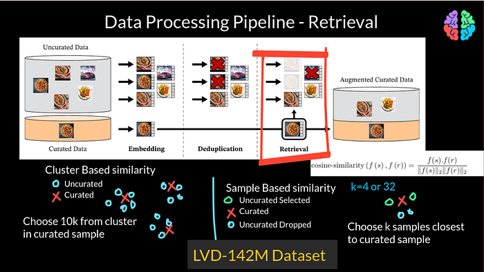
They then use retrieval to find images similar to a given image in the curated dataset. More specifically, they use 2 types of similarity namely — sample-based similarity and cluster-based similarity. For both the types, they use cosine similarity to measure the similarities. For the sample based, they sample k uncurated images nearest to a given curated image and include those that are more than a similarity threshold and discard the rest. They use k=4 and k=32 in the process. Then there is cluseter-based retrieval where they cluster the uncurated data into different clusters and from each cluster, they sample 10,000 images and discard the rest. After doing these steps, by the end of the retrieval process, the resulting dataset had 142M images resulting in the LVD-142M images dataset.

Discriminative self-supervised pretraining

Beyond that pipeline to generate the training dataset, DINO-v2 is a series of improvements to DINO-v1. I have done a separate video on DINO-v1 but just for completion let me brief here. DINO stands for self-distillation with no labels. We start the training with two variations x1 and x2 of the same image x and pass it through separate student and teacher networks whose architecture is the same but we train them differently. When I say differently, we train the student network with the cross entropy loss However, there is a stop gradient preventing the training of the teacher network with this loss. But the teacher network is updated with an exponential moving average. We can call this training as having image level objective because we use the entire image for training throughout.

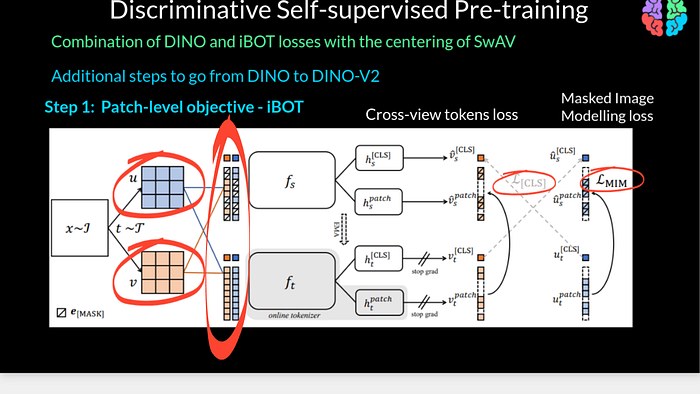
The first improvement over DINI-v1 is to introduce patch level objective from iBOT. Given an input image x, we now extract two views u and v and for each view we extract patches instead of working with the entire image. We introduce two losses namely cross-view tokens loss which is the same as cross entropy in DINO-v1 but this time we pass masked patches to the student and pass the unmasked patches to the teacher network. Its somewhat like the teacher sees all the information, but as the student is learning, the sutdent has to guess the missing pieces of the puzzle. The second loss is the masked image modelling loss between the masked and unmasked outputs from the student and teacher respectively.

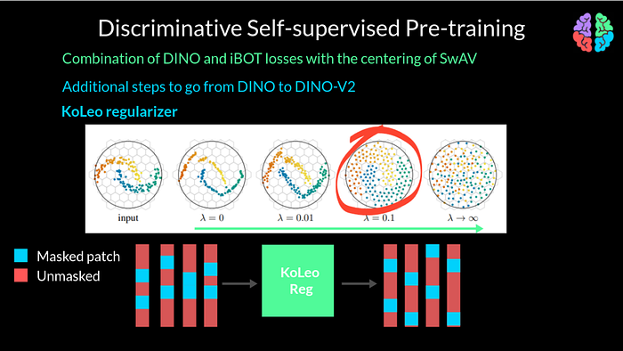
In addition to the patchwise objective, they also introduce a KoLeo Regularisation to the loss. To undertand KoLeo Regularization, lets take a look at this figure. Like any other regularization, it has a paramter lambda. By increasing the parameter lambda, the features can be made to spread across the manifold compared to the input. In our problem, because we extract patches to work with, if you take a batch of say 4 images and their corresponding masked tokens, the masking shown in blue here may not be distributed well enough in the batch. The masks may be distributed, lets say somewhere at the center or at the top or even bottom of the features. To overcome this, KoLeo regularization introduces uniform spanning of the masked patches across the input and across a given batch of inputs. In this example, the batch size is 4. As a last additional improvement, they also increase the resolution of the training images to 518 X 518 towards the end of pretraining.

Effective Implementation

Now that we know we train with a massive training dataset and some improvements to DINO-v1, we also have to make sure that the implementation is quite efficient. The first step towards efficiency is flash attention instead of the standard attention in the self-attention layers. The next step would be to introduce nested tensors in order to process the global crop and the local crops of the image together rather than process them separately. They have also leveraged the Fully-Shaded Data Parallel available to shard the models across GPUs which is available from PyTorch 2.0. And lastly they have also used model distillation to distill the very large ViT-G to other smaller models like ViT-L.

With all these shiny new improvements to DINO, the results do indeed look impressive with DINO-v2 performing better than iBOT in segmentation in every single dataset. When it comes to depth estimation, it once again outperforms iBOT in quite common datasets like KITTI and NYUd.

I hope you enjoyed that. I will see you in my next …