ControlNet — Take complete control of images from the generative model

This week let's look at one of the most influential papers of 2023 - ControlNets!
When we take image generation models such as Stable Diffusion, the quality of the image generated is mind-blowing. However, the output is pretty much controlled by text input, which is a prompt. Text inputs are quite limited in their ability to control the output.
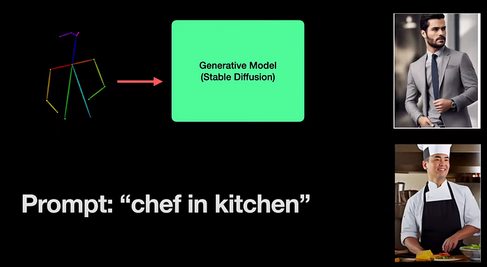
For example, If I want to generate an image of a man standing in the pose above, I can not imagine how many words we need to define this pose. But if we can feed this pose directly to the model, then it makes our jobs much easier. If we can feed a text prompt (“chef in the kitchen”) along with the pose, then we have even better control and we can generate the image of a chef standing in the same pose.
This problem of precisely controlling the spatial layout of the generated images, through input images is what is addressed by ControlNet. The inputs could be sketches, normal maps, depth maps, edges, segmentation masks, and human poses.
No wonder ControlNet got the prestigious Marr Prize at the ICCV conference in 2023. The impact on the community can be already felt by over 730 citations to the paper.
So in this article, let's look at the controlnet architecture, the zero initialization technique, and the qualitative results along with some ablation studies. So without further adieu, let's get started.
Visual Explanation
If you are like me and would like a visual, animated explanation of ControlNet, then you may choose to watch the below video:
ControlNet Architecture
We all know that neural networks are composed of several neural network blocks. For example, if you take the famous ResNet, it has several ResNet blocks in sequence. Similarly, the famous transformers have a sequence of multi-headed attention blocks.
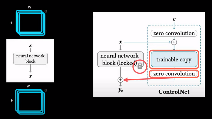
To understand the controlnet architecture, let's consider a single block of any neural network from a generative model, say Stable Diffusion, it typically takes a 3 dimensional tensor with height width, and number of channels as input and outputs a similar dimensional tensor. To add ControlNet to this block, we first make a copy of the weights of the block and freeze the actual weights. This trainable copy is then connected to zero convolution and the output of zero convolution is sent back as input to the frozen block. So whenever we train the model, it's this trainable copy that gets updated but the actual pre-trained generative model remains frozen.
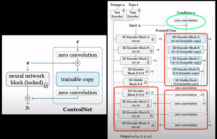
Scaling up this idea to stable diffusion, which has encoder and decoder layers, the blocks in blue are the trainable copies of the encoder layers. The output of each of these blocks is put through the zero convolutions which in turn are fed into the stable diffusion decoder blocks. One more place where zero convolutions are used is when we take the input conditioning such as the depth map or the pose and combine them with the input represented as z_t.
Talking of zero convolutions, these are simple 1 by 1 convolutional layers whose weights and biases are initialized to zero.
Bridging Control and Feature space
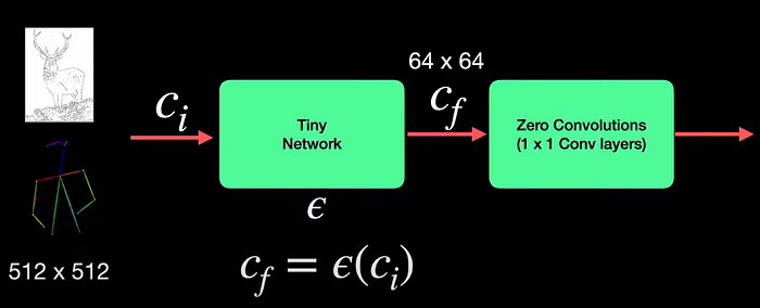
The conditioning inputs which are edge maps or poses have a dimension of 512 by 512, which proves to be a very high dimension for these 1 by 1 convolution layers. So to overcome this, a tiny neural network with 4 conv layers is introduced which converts these images from the image conditioning space c_i to the feature conditioning space c_f thereby reducing the dimension to 64 by 64. All that it means is that the dimension of the conditioning is small enough to be happily used with zero convolutions.
Whenever there are optional text prompts c_t as conditioning input, they are taken care of by CLIP encoders along with positional encoding for time and are fed directly to the frozen weights of the stable diffusion model.
Training Process
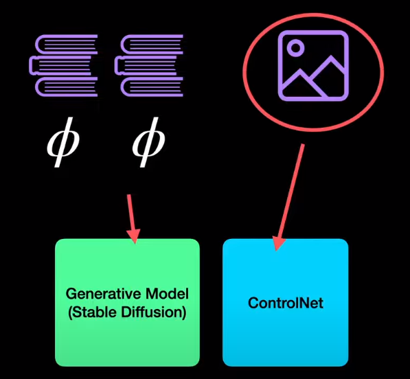
When training ControlNet, we would like to introduce image prompts instead of text prompts to shift the control from text to image prompts. So, we deliberately replace half the text prompts in the training data with empty strings. So the network is now forced to learn the semantics of the conditioning images such as edges, poses, or depth maps.
Training this way, the model abruptly succeeds in following the input conditioning image; usually in less than 10K optimization steps. This phenomenon is referred to as the “sudden convergence phenomenon”.
For example, we can notice in the paper that around step 6100, though the output is an apple the spatial layout of the apple is quite different from that of the input edge conditioning in the test image. But suddenly after 8 thousand steps, we can see the spatial semantics are obeyed to the dot. And at 12 thousand steps, it's only getting better at matching the semantics of the input image prompt.
With that trained model, if we move on to inference, ControlNet introduces what is called Classifier-free guidance resolution weighting. Now that's a mouthful. So let's break it down and start with Classifier guidance. Then move on to classifier-free guidance and then resolution weight.
Classifier guidance
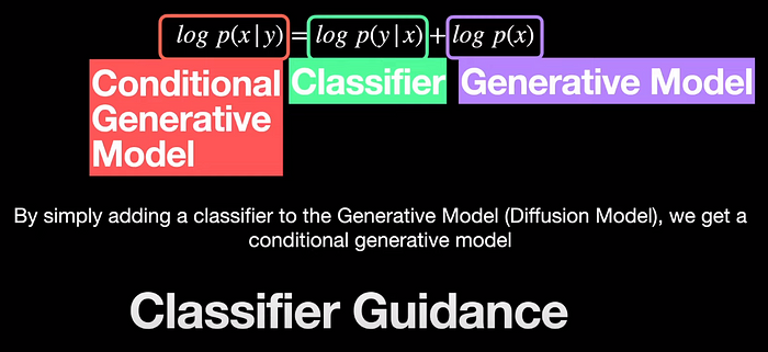
To understand classifier guidance, let's get slightly mathematical and begin with the well-known Bayes’ Theorem. By simply applying log to the equation, we can convert multiplications to additions and divisions to subtractions. So the modified equation becomes this. Lastly, assuming that the distribution of the labels p(y) is trivial or if we take them for granted, we can set it to zero. And so we arrive at this simplified equation.
Let's break this down to see what each of the terms represents. The rightmost term is simply the distribution of the input data x. In other words, it is a generative model because if we simply sample from this distribution of x, we can get outputs similar to that of x. The middle term represents a discriminative classifier as it says, given an input x, give me the probability of the class y. The leftmost term is the conditional generative model as it says, given a label y, give me a generated sample x from the distribution.
So long story short, by simply adding a classifier to the Generative Model (Diffusion Model), we get a conditional generative model. This is the exact idea of classifier guidance.
However one of the drawbacks of this classifier is that it needs to be trained with noise input; because the input to the diffusion model is noise. And so the classifier needs to take the noise sample and classify what class that noise belongs to. The solution to this problem however is to get rid of the classifier altogether and arrive at classifier-free guidance.
Classifier-free guidance
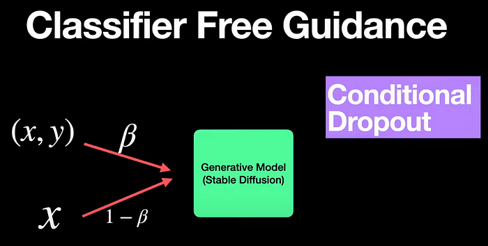
We get rid of the classifier by the idea of conditioning dropout. So we train a conditional diffusion model such as Stable diffusion with and without the conditioning labels y. And we strike a balance between the two using a weighting factor, say beta. And we set it in such a way that the conditioning y is removed about 20% of the time.
Papers like GLIDE from OpenAI used this idea of classifier-free guidance to generate images like these for an input prompt, “A stained glass window of a panda eating bamboo”
Classifier-free guidance Resolution Weighting
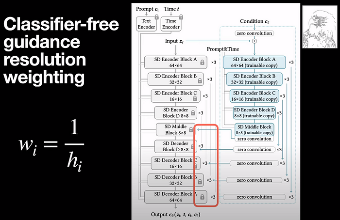
Getting back to ControlNet, ControlNet refines the idea into Classifier-free guidance resolution weighting. Because ControlNet has two networks, the diffusion model and its trained copy, the ControlNet, whenever we have a conditioning image, say an edge map, we introduce additional weights that are multiplied at the connection between the diffusion model and the ControlNet so that the output is much more refined. These are not neural network weights, but simple numbers multiplied at each stage. The weights are inversely proportional to the size of the blocks h_i we are connecting into.
The results indicate that by using this resolution weighting, shown as “full without prompt” on the right, we are getting the best results compared to being generated without the weighted guidance
Ablation Studies

In terms of ablation studies, they branch off into two and study the effect of network initialization and the input prompt settings. For initialization, they try standard initialization of the weights with Gaussian instead of zero convolutions. Row b shows the results with Gaussian initialization. And the quality of images is worse than using zero convolutions. Similarly, they trained with a light version of the ControlNet (ControlNetLite) by replacing the copy of the weights with simple convolutions to see if the ControlNet can be lightweight.
The authors also tried challenging prompting scenarios such as no prompt, insufficient prompt, and conflicting prompts. And in all scenarios, ControlNet manages to generate reasonably meaningful images rather than collapsing.
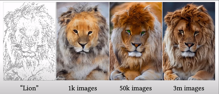
They also study the dataset size that is needed to train ControlNet and show that even though we can get reasonable outputs with just 1 thousand images, we can see that with a lot more images, say 50 thousand, the results look better and they get even better with 3 million training samples.
Lastly, ControlNet is not just restricted to stable diffusion, but can also be applied to other generative models like Cosmic diffusion and protogen.
So to wrap things up, these are the variety of control images you can provide as input prompts along with the generated images for each of them. It includes sketches, normal maps, depth maps, edges, and human pose.
With that, I think we have covered everything that I wanted to say about controlNet. Hope that gives enough insight about controlNet.
I hope to see you in my next. Until then, take care…
