What are AutoEncoders in Deep Learning?

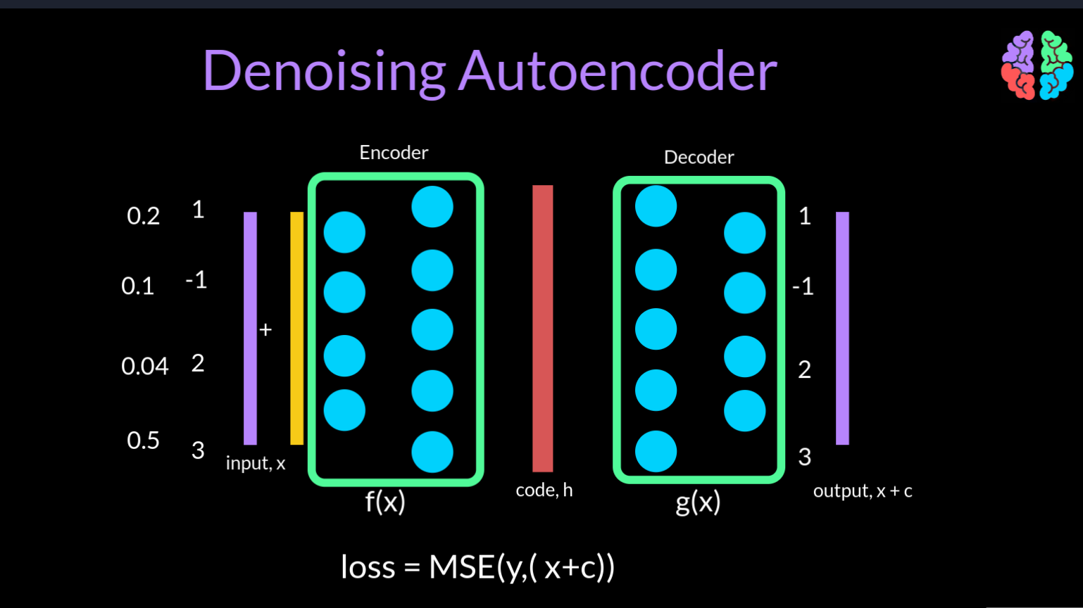
Autoencoders consists of 2 parts — the encoder and the decoder . The encoder takes the input and outputs what is called the “code” . The decoder takes this code and is trained to convert it back into the input . If we go by the traditional argument that neural networks are function mappings, then the encoder can be f(x)  and decoder can be g(h) . So our finaly output y is g(f(x)). As we are only training these networks to reproduce the input data x, they don’t need any labels or in other words they are unsupervised neural networks.

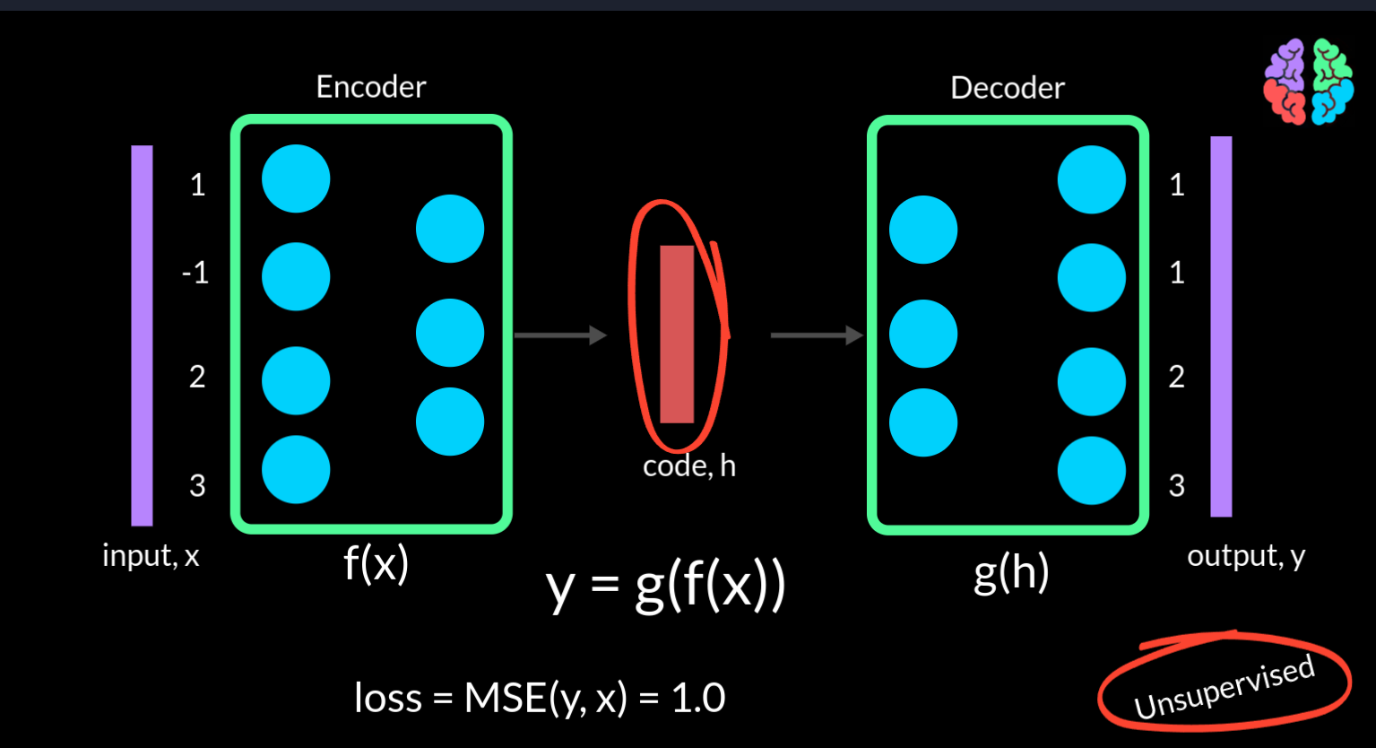
If we take a simple example of the input to be a 4 dimensional vector of values say 1, -1, 2, 3,  and if the output from the network is 1, 1, 2, 3,  we can compute a simple mean squared loss during training, which is 1 in this example and minimise this loss to train the network.
You may now start to realise that the network can quickly learn the unity function and the output can be the same as the input . However, the dimension of the code comes to the rescue. Note that in this figure that the output dimension of the encoder is just 3 implying that the dimension of the code is also 3  compared to the input dimension 4. This means that the network should somehow figure out a way to squeeze the 4 dimensiona l input into a 3 dimensional space. Using the same example input <click>, the code will be a completely different representation with values say 0.8, 1.2 and 2.2. By doing this, the encoder has literally encoded the input to a lower size. This autoencoder where the dimension of the code is less than the dimension of the input, its called an undercomplete autoencoder
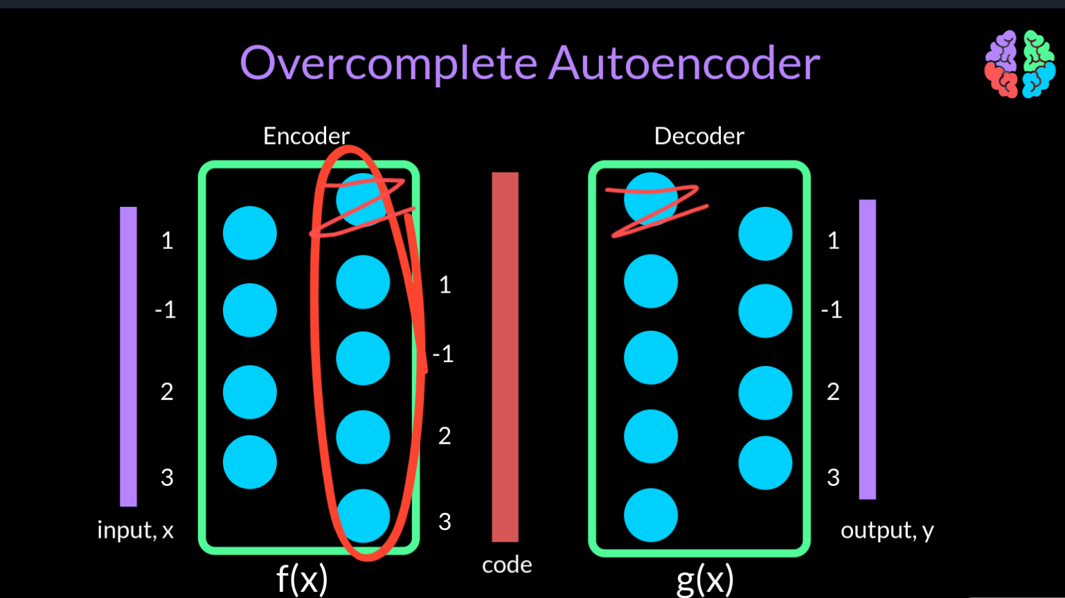
Arguing the same way, if the dimension of the code is equal to or larger than the dimension of the input (in this case 5), then its a overcomplete autoencoder . Whenever the autoencoder is overcomplete, there is a very high chance that it maps to unity during training. In other words, it starts sending the input directly to the output by simply ignoring the additional nodes in the network.

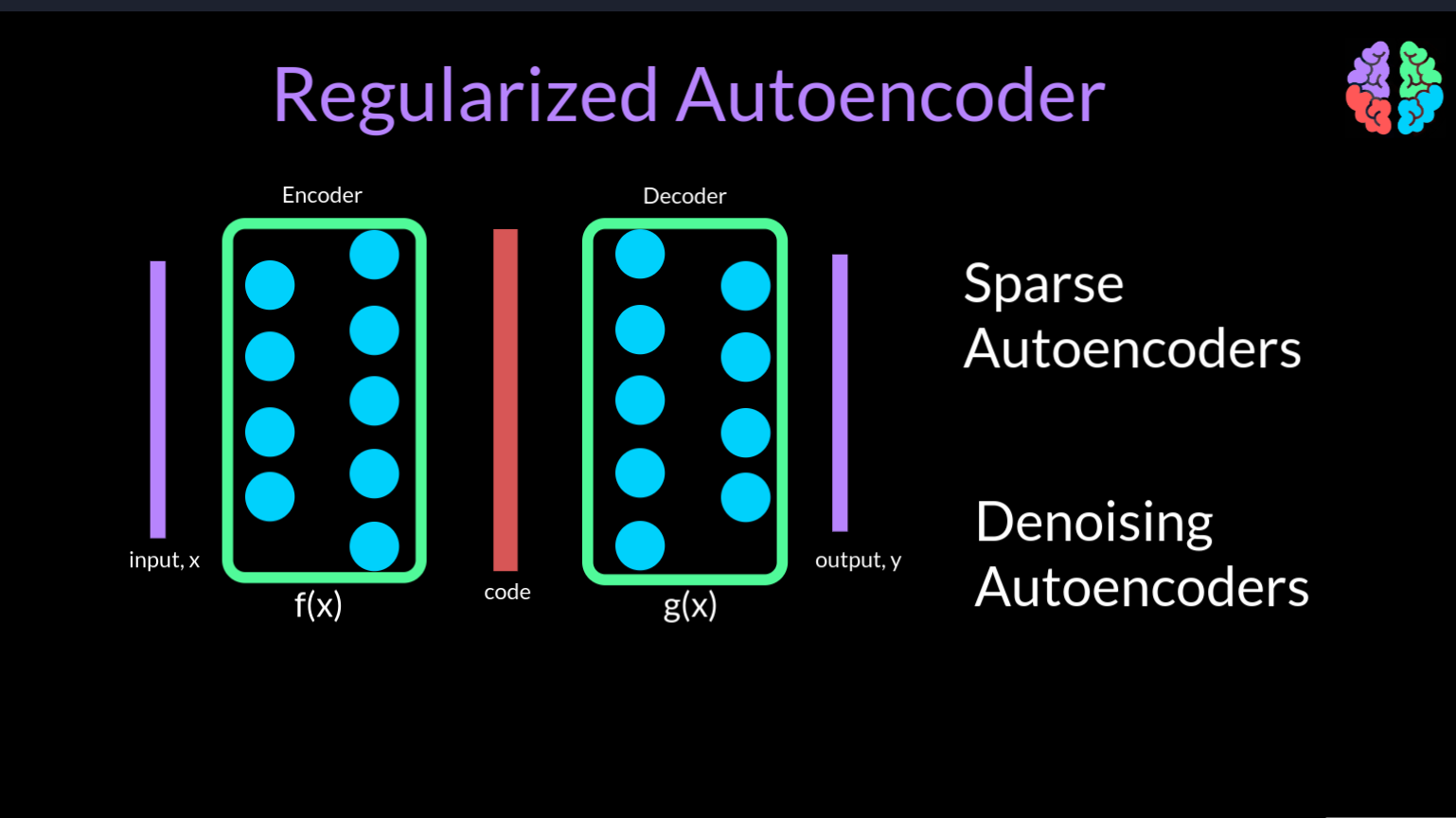
There are two ways we could overcome this problem. One is by introducing sparsity in the network and these are called sparse autoencoders. The other way is to introduce noise into the network and this gives birth to the class of denoising autoencoders. Both these types are grouped under the name reguliarzed autoencoders. Now lets look at each of them.

To understand sparse autoencoders, lets assume the scenario where the autoencoder learns unity and literally passes the input to the output. This scenario can be fixed by simply setting some of the values of the hidden code to zeros. By this simple fix, the network behaves as if it is now an undercomplete autoencoder.

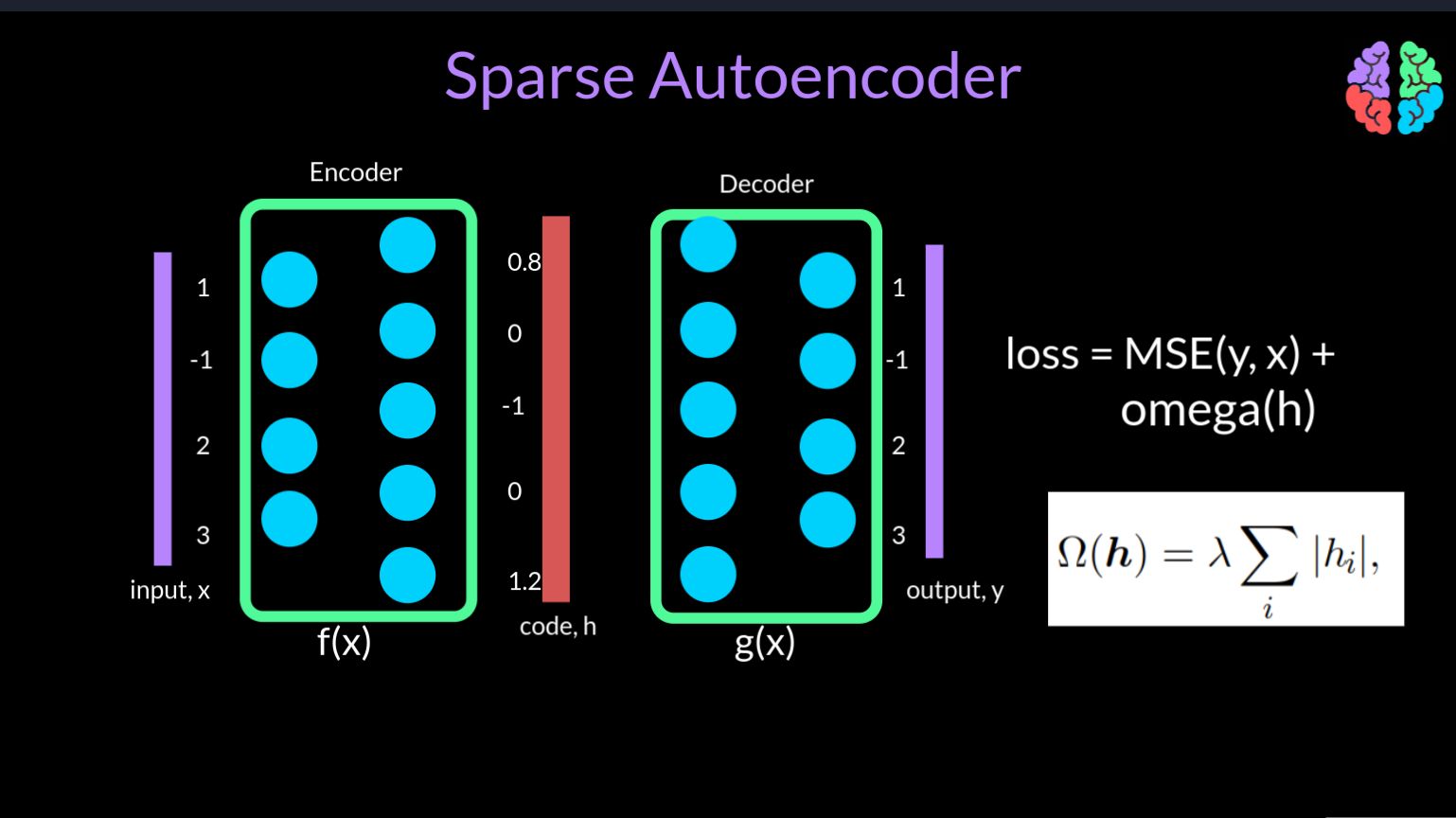
But how do we force this during training? Lets go back to our mean squared error loss betwen the input and the output. We now introduce a new loss function omega that is acts on the code h. This is similar to L1 regularisation which is used to reduce the overfitting. But in this case the new term omega forces the codes to turn off a few values or in other words introduces sparsity in the network.

A diferent solution to fix the copying problem is to corrupt the input by adding some random noise during training and show the uncorrupted input as the output. This type of autoencoders is called a denoising autoencoder. As they learn to remove the noise from the input. In terms of the mean squared error loss function, the input is not x but x+c where c is a corruption noise vector whose size is the same as that of the input.

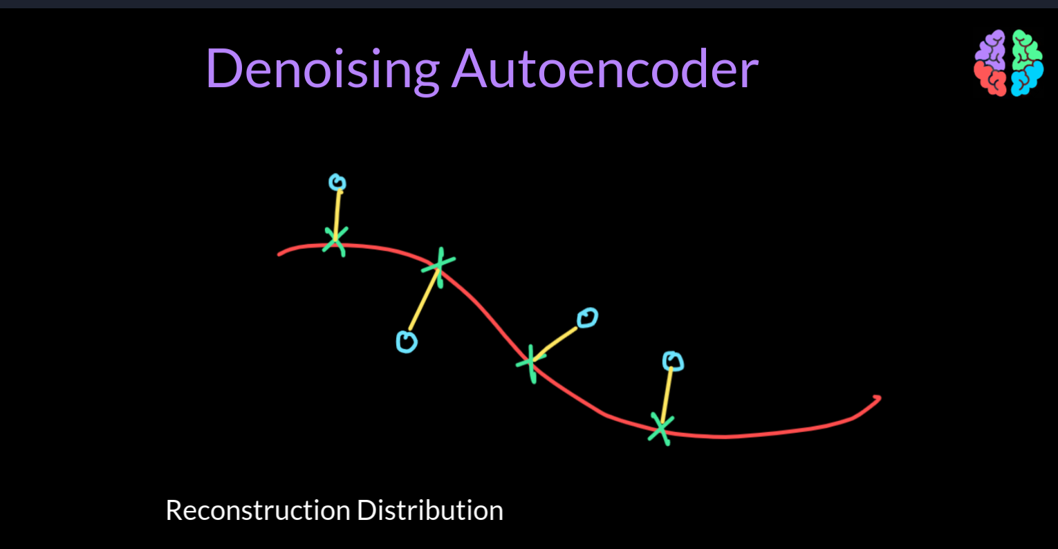
Just to visalize what is going on, if we take this red line as the manifold representing the real data points shown in green and the points in blue circle are the corrupred data points, then the autoencoder is learning a vector field around the manifold shown with yellow. In other words the denoising autoencoder learns the reconstruction distribution rather than the distribution of the data itself.

Applications of AutoEncoders

In terms of the applications of autoencoders, clearly copying the input to the output is not useful. What is indeed useful is the learnt hidden representation of the input in a lower dimensional code, h. These hidden representations can now act as features embeddings from the input. Traditionally autoencoders have been used for dimensionality reduction where we reduce the inputs to the codes and work with the codes for training the models instead of the inputs thereby leading to less memory and faster runtime for the models.
A useful byproduct of dimensionality reduction is information retrieval. Because we can reduce the input to lower dimensional space, we can even store them in hash tables and use these tables to retrieve information whenever they are queried.

The last but the most exciting application of autoencoders is for generating data and the type of autoencoder used for generating data is called Variational Autoencoders. I will go explain them in my upcoming post. Till then stay tuned.

Shoutout

Why not checkout out YouTube channel AI Bites where we explain AI concepts and papers clearly.

Why not subscribe to our newsletter to get similar articles right to your inbox.

I will see you in my next...