Comparing Kolmogorov-Arnold Network(KAN ) and Multi-Layer Perceptrons (MLPs)

We have taken the classic Multi-Layer Perceptrons (MLPs) for granted and built so many architectures around it. MLPs are part and parcel of every single LLM or foundation model that we see today such as chatGPT, LLAMA, DALLE, and CLIP. Or even simple recognition models such as YOLO-v*.
What if I now tell you that we have a competitor for the very MLPs? There is a new paper in town called the “Kolmogorov-Arnold Network” or KAN in short which challenges the MLPs. If the solution they are proposing truly scales, then we can have the next generation of neural networks which will take us yet another step closer to Artificial General Intelligence(AGI).
While the MLPs comprise activation functions such as ReLU, sigmoid, tanh, GeLU, etc., KAN proposes that we learn these activation functions. So, how does KAN do it? What's the mathematics behind it? How is it implemented? and how do we even train KANs?
I have tried my best to summarise the KAN paper here. You can either choose to read this gist or read the paper which is 48 pages long!
Visual Explanation
If you are like me and would like to visualize things to understand better, here is a video form of this article:
MLPs — The problem
Let’s start with MLPs which we are quite familiar with. The MLPs are composed of nodes and edges. In each node, we have the inputs being summed and activations such as ReLU, GeLU, SeLU applied in order to produce the output for that particular node.

These activation functions never change during the training process. In other words, they don’t have any parameters. They are not intelligent enough to tune themselves to a given training dataset. So what gets trained or updated during training is the weights at each of these nodes.
Now, what if we question the assumption that the activation function needs to be fixed and make them trainable? So, that's the challenge the KAN network tried to address. The activation functions of the KAN network get updated during the training process. Before we delve any deeper, let's start with polynomials and curve fitting.
Polynomials and Curve Fitting
So, the fundamental idea of KANs is that any multi-variate composite function can be broken down into a sum of several functions that are single variables.

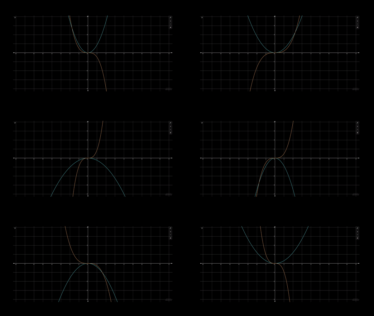
For example, let's say we have an equation of degree 3 where y=x³ as plotted by the yellow curve above. And another equation of degree 2, y=x², as shown by the blue curve in the above animation. We can see in this visualization that using x², can never achieve the curvature achieved by x³.
Let's assume we are given the data represented by the red and blue points below and we wish to find the binary classification boundary between the two classes.

Using a second-order polynomial, x², we won’t be able to find the boundary between the two as the x² curve is “U” shaped but the data is “S” shaped. Though using x³ is apt for this data, it comes with an extra computational cost. A different solution could be to use x² when input x is negative but use -x² when x is positive (blue curve drawn with hand in the above figure).
All that we have done is add two lower-degree polynomials to achieve a curve with a higher degree of freedom. This is the exact idea behind KAN networks.
A toy Problem
Let’s now take a slightly more sophisticated toy problem where we know that the data is generated by a simple equation, y=exp(sin(x1² + x2²) + sin(x3² + x4²)). So we have 4 input variables and we have three operations namely, exponent, sine, and squared. So we can choose four input nodes with three layers, each dedicated to the three different operations as shown below.

After training, the nodes will converge to squared, sinusoid, and exponent functions, to fit the data.
As this is a toy problem, we know the equation from which the data came from. But practically, we don’t know the distribution of real-world data. One way to address this problem is by using the B-splines.
Splines and B-splines
The fundamental idea of B-splines is that any given function or curve can be represented as a combination of simpler functions or curves. These simpler functions are called basis functions. For example, let's take the red curve in the below figure. For the sake of simplicity, let's try to represent this with just two basis functions.
We can break it down into 3 points as we are going to represent it with the sum of two basis functions. These points are called knots. There can be any number n of basis functions. The parameter that controls how this basis functions combinations is c. There can be discontinuities at knots when we “join” two curves. The solution is to constrain the curvature of the curves at the knots so that we get a smooth curve. For example, we can constrain the slope of the two curves to be the same at the knots, as shown by the green arrow in the below figure.

As we cannot impose such a constraint in the neural network, they have introduced Residual Activation Functions in the paper. This acts more like a regularization. Practically, this is the SeLU activation that is added to the standard spline function as seen in the paper below.

Spline Grids and Fine-Graining of KANs
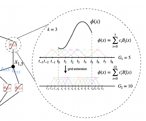
KANs introduce a new way of training called fine-graining. What we are all familiar with is fine-tuning where we either add more parameters to the model. But in the case of fine-graining, we can improve the density of grids in the spline grids. This is what they call grid extension.

As we can see from the figure above from the paper, fine-graining is simply making the grids of B-splines dense so that they become more representative and hence more powerful.
Computational Complexity
One of the disadvantages of splines is that they are recursive and so computationally expensive. Their computational complexity is O(N²LG) which is higher than the usual complexity of O(N²L) for MLPs. The additional complexity comes from the grid intervals G.
The authors defend this inherent problem by showing that:
- the number of parameters needed by KAN is less compared to MLPs for the same problem
- KANs converge quickly and efficiently during training thereby needing less training time
We will see the plots of these defenses in the results section. For now, let's look more into another specialty of KANs.
Interpretability and Choosing KAN Layers
As KANs learn functions, it's not simply a black box like MLPs where we can simply design them by choosing the depth and width of the MLP for a given data or problem. So to make KANs more interpretable and to design a good KAN network, we need to follow the below steps:
- Sparsification. We start with a larger-than-anticipated KAN network and introduce regularization by introducing the L1 norm of the activation function instead of the inputs as we generally do with Machine Learning.
- Pruning. Once the sparse network is trained, we can then remove unnecessary nodes that are below a certain threshold in a set criteria or score.
- Symbolification. When we vaguely know what function constitutes a given data, we can set a few nodes to take that function. This is called symbolification. For example, if we work with sound waves, most of the data is sinusoidal and so we ease our lives by setting some of the nodes to be sinusoids. The framework enables us to do so by providing an interface function called,
fix_symbolic(l,i,j,f)where l, i, j are node layer and locations and f is the function that can besine, cosine, log, etc

The different steps have been summarised in the above figure. We start with a large network and sparsify(step 1), prune the resulting network (step 2), set some symbolification (step 3), train the network (step 4), and finally arrive at the trained model.
Experiments and Results
Using the steps mentioned above, they have trained KAN networks for five different toy problems to illustrate their effectiveness and compare them against MLPs. The key takeaways from the comparison are:
- KAN trains much faster than MLPs, thereby compromising the computational complexity inherent to it.
- KAN can do with fewer parameters what MLPs can do with much more
- KANs converge very smoothly with fast decreasing loss compared to MLPs
The first point is depicted by the thick blue line in the five plots in the top plot above for the 5 toy problems. The last two points are illustrated by the plot at the bottom showing loss curves and the parameter counts to solve any given problem.


Catastrophic Forgetting
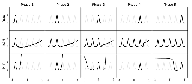
The next takeaway is that KANs are far better than MLPs in the catastrophic forgetting problem. If we feed sequence data for continual learning, KANs seem to remember the past data far better compared to MLPs. This is shown in the figure below where KAN reproduces the 5 phases in the data but MLP struggles.

Other results
They have also done extensive experiments to show that KAN can be used for problems involving partial differentials and Physics equations. Rather than going into those details, let's look at when to choose KANs versus MLPs.
Choosing between KAN and MLP
They have given the below figure to guide us on when to choose KANs over MLPs. So, choose KANs if,
- you are dealing with structural data like waveforms or graphs
- wish to have continual learning from data
- don’t care much about the training time!
- high dimensional data

Otherwise, MLPs still win.
Discussion and Conclusion
In my opinion, KANs are not here to replace MLPs as to how transformers cleanly swept the NLP landscape. Rather, KANs will prove handy for niche problems in mathematics and physics. Even then, I feel we need many more improvements. But for big-data problems that are solved with foundation models, KANs have a long way to go, at least with their current state.
Furthermore, the training approach and designing KAN architecture tends to deviate from the standard way of designing and training modern-day neural networks. Nevertheless, the GitHub page already has 13k stars and 1.2k forks, indicating it is up for something.
Let's wait and watch this space...
